
FNCE102 FMI
In this post, I’ll be focusing on the module Financial Markets & Investments (FMI). This post will consist a comprehensive interactive study guide I built to consolidate my understanding of the module.

After completing my Year 2 Semester 2, I've gained a lot of new and well-rounded knowledge. There's no better time to consolidate what I've learned than now. This post covers all 12 lectures: from capital allocation and portfolio theory, to derivatives, bonds, and performance evaluation. It is filled with concept explanations, worked examples, formula references, practice questions, and interactive calculators. Hope this is useful for whoever is trying to grasp an understanding of this module.
Disclaimer: This post reflects my personal experience with the module during the term from January to May 2026, as taught by this specific professor.
Financial Markets
& Instruments
A comprehensive self-study hub. Theory, solving guide, formulas, and exam strategy in one place.
The Big Picture — How Everything Connects
Roles of Financial Markets
Stock prices reflect firm prospects. Capital flows to companies with best outlooks. When the market is optimistic, stock price rises — prices aggregate dispersed information.
Move purchasing power across time. Use securities to store wealth in high-earning periods; sell in low-earning periods. Separates earning from consumption.
Wide variety of securities lets investors select those matching their risk appetite. This benefits issuers who can then issue at best possible prices.
Enables large-scale enterprise. Agency problems arise when managers pursue own interests. Mitigated by: compensation plans, board monitoring, analyst scrutiny, takeover threats.
Four Market Types
| Market | What Trades | Examples |
|---|---|---|
| Fixed Income | Debt instruments | T-bills, T-bonds, corporate bonds |
| Equity | Ownership stakes | Common & preferred stock |
| Forex | Currencies | Exchange rates, forwards |
| Derivatives | Derived value | Futures & forwards (covered here); Options (separate topic) |
Fixed Income: Money Market vs Capital Market
- Treasury Bills: Government-issued, discount basis. Highly liquid. No coupons — investor earns from discount to par.
n = days to maturity, r = rate (decimal)
E.g. n=109, r=0.00298: Price = 100 − (109×0.00298)/360 = 99.91
- T-Notes: maturity up to 10yr; T-Bonds: 10–30yr; semiannual coupons; par = $1,000
- Corporate Bonds: higher default risk; secured (collateral) vs debentures (no collateral); callable / convertible
- Mortgage-Backed Securities: proportional ownership of a mortgage pool; securitised
Singapore Bond Market
| Instrument | Tenor | Interest | Min. Inv. | SGX-Tradable? |
|---|---|---|---|---|
| T-Bills | 6 months or 1 year | Discount basis | S$1,000 | Yes |
| SGS Bonds | 2–50 years | Fixed semiannual | S$1,000 | Yes |
| SSBs | Up to 10 years | Fixed step-up semiannual | S$500 | No (redeem via MAS) |
- Retail Bonds: all investors, min S$1,000
- Wholesale Bonds: institutional & accredited investors only, larger amounts
- Seasoning Bonds: wholesale bonds that meet eligibility criteria, offered to retail after 6 months SGX listing, min S$1,000
Approved financial institutions (banks) that facilitate MAS auctions for Singapore Government Securities. They submit competitive bids and distribute bonds to investors, ensuring liquidity in the government bond market.
Equity Securities
| Common | Preferred | |
|---|---|---|
| Ownership & voting | Yes — residual claim | No voting rights |
| Dividends | Variable, discretionary | Fixed (like perpetuity) |
| Priority in liquidation | Last | Before common |
| Liability | Limited | Limited |
Dividend Yield = Annual Dividends / Purchase Price
P/E Ratio = Price per Share / Earnings per Share
| Index | Method | Notes |
|---|---|---|
| DJIA | Price-weighted | 30 blue-chips; since 1896 |
| S&P 500 | Market-value-weighted | 500 firms; broader |
| STI | Market-cap-weighted | Singapore benchmark |
Forex: Law of One Price
Exchange rates fluctuate due to differences in price levels (inflation) and interest rates across countries.
If Japanese prices then rise to JPY250: New equilibrium = US$1 = JPY125. Japanese inflation → JPY depreciates, US$ appreciates.
ERSG — Ethics, Social Responsibility, Sustainability & Governance
ERSG trends are reshaping financial markets and investment decisions. Knowing them is increasingly essential for investors.
- Ethics: Moral principles guiding unbiased, non-prejudiced decisions
- Social Responsibility: Entities responsible for societal benefit, not just individual gain
- Sustainability — Environmental: Preserve environment for future generations; anti-pollution, climate risk
- Sustainability — Business: Resilience in face of disruptions (Covid-19, geopolitical risks, tech changes)
- Transparency
- Responsibility
- Accountability
- Fairness
- Risk Management
Concern: conflict between shareholders’ and managers’ interests. Corporate governance rules help ensure markets are efficient avenues for capital allocation.
Risk Aversion & Utility
A > 0 → Risk-averse (penalises risk) ← normal
A = 0 → Risk-neutral (ignores risk)
A < 0 → Risk-lover (enjoys risk)
Risk-free: U = rf (sigma = 0, no penalty)
| Speculation | Gambling | |
|---|---|---|
| Risk premium | Positive | Zero (fair game) |
| Expected profit | Positive | Zero |
| Risk-averse accept? | Yes | No |
A coin flip = gambling (p=0.5 each side, expected profit = 0). But if you believe p > 0.5 (heterogeneous expectations), it looks like speculation to you.
Mean-Variance Criterion
Portfolio A dominates Portfolio B if E(rA) ≥ E(rB) and sigmaA ≤ sigmaB, with at least one strict inequality.
- Quadrant IV portfolios (lower E(r), higher sigma than P): dominated by P — always avoid.
- Quadrant I portfolios (higher E(r), lower sigma than P): dominate P — always prefer.
- Quadrants II & III: neither clearly dominates. Use indifference curves to decide. Portfolio must lie northwest of P to be superior.
Measuring Risk Aversion (KYC)
Financial advisers gauge risk aversion by:
- Questionnaires — score various risk scenarios
- Observing decisions when confronted with risk
- Observing how much people are willing to pay to avoid risk
Capital Allocation Line (CAL)
Mix risky portfolio P (proportion y) with risk-free F (proportion 1−y).
sigmaC = y × sigmaP
E.g. rf=7%, E(rP)=15%, sigmaP=22%:
y=0.5: E(rC)=11%, sigmaC=11%
y=1.4 (leverage): E(rC)=18.2%, sigmaC=30.8%
= reward per unit of total risk
ALL points on the CAL share the same Sharpe ratio — leverage does not improve Sharpe, only scales it.
CML = special CAL using the market portfolio.
Example: Portfolio Z (Asset Allocation)
Total portfolio Z = $300,000. Currently: 30% in risk-free F ($90,000), 70% in risky P ($210,000). Within P: 54% stocks ($113,400), 46% bonds ($96,600).
Optimal Allocation y*
y* ↑ when: risk premium ↑, A ↓, sigmaP ↓
y* > 1 → Leverage (borrow to invest >100% in P)
y* < 0 → Short the risky portfolio
E.g. rf=7%, E(rP)=15%, sigmaP=22%, A=4:
y* = (15%−7%) / [4 × (0.22)²] = 0.08/0.1936 = 0.413
Indifference Curves
An indifference curve connects all (E(r), sigma) pairs giving the same utility score. To build one:
- Start with risk-free: U = rf (sigma = 0)
- Increase sigma. Solve for E(r) that maintains same U: E(r) = U + ½Aσ²
- Repeat for all sigma values → plot pairs
Two Types of Risk
Marketwide risk sources. Remains even after diversification. Also called: non-diversifiable. Eg. GDP, interest rates, global financial crises. Investors are compensated with the market risk premium.
Risk unique to a firm or industry. Eliminated by holding many uncorrelated securities. Also called: diversifiable or nonsystematic. No compensation — investors can diversify it away for free.
Two-Asset Portfolio Formulas
Unaffected by correlation — always weighted avg.
+ 2×wD×wE×Cov(rD,rE)
Cov(rD,rE) = rho × sigmaD × sigmaE
Effect of Correlation
| Correlation rho | Portfolio SD | Benefit |
|---|---|---|
| +1 | = weighted avg of SDs | Zero — no diversification |
| 0 to +1 | < weighted avg | Partial benefit |
| 0 | Significantly lower | Good benefit |
| −1 | Can reach zero! | Maximum benefit (perfect hedge) |
E.g. sigmaD=12%, sigmaE=20%: wD=20/32=62.5%, wE=12/32=37.5% → sigmaP=0
Minimum Variance & Tangency Portfolio
wE = 1 − wD
Minimises sigma. Does NOT maximise Sharpe ratio.
wD = [E(RD)×sigmaE² − E(RE)×Cov] / [E(RD)×sigmaE² + E(RE)×sigmaD² − (E(RD)+E(RE))×Cov]
The optimal risky portfolio P is the same for ALL investors regardless of risk aversion. Only y* differs. One mutual fund can serve many clients — everyone holds P in different proportions combined with the risk-free asset.
Core Equations
Ri = excess return of security i (= ri − rf)
RM = excess return of market index
alpha_i = nonmarket expected excess return (stock-specific premium)
beta_i = systematic sensitivity to market; uncorrelated with ei
ei = firm-specific residual (mean=0, uncorrelated with market)
Variance Decomposition
Systematic: beta_i² × sigmaM² ← non-diversifiable
Firm-specific: sigma²(ei) ← diversifiable
R² = beta_i²×sigmaM² / sigma_i² (systematic proportion)
ALL covariance comes ONLY from the common market factor. Firm-specific residuals are mutually uncorrelated — this is the key simplification of the SIM.
Diversification Under SIM
For an equally-weighted portfolio of n stocks: portfolio’s excess return RP = alphaP + betaP × RM + eP
Systematic (betaP²×sigmaM²): persists regardless of n
→ Non-diversifiable
As n → ∞: sigma²(eP) → 0
→ Diversifiable — cancels out!
Beta, Adjusted Beta & Alpha
| Beta | Meaning | Examples |
|---|---|---|
| beta = 1 | Moves with market | Index fund |
| beta > 1 | Amplifies market (cyclical) | Ford ~1.33 |
| beta < 1 | Defensive, less sensitive | Utilities, staples |
| beta = 0 | No systematic risk | T-bills |
Betas revert toward 1 over time.
E.g. Historical beta = 1.9:
Adj beta = 2/3×1.9 + 1/3×1.0 = 1.6
Use E(r) = rf + 1.6×[E(rM)−rf]
Expected Return-Beta Relationship
Taking expected values of Ri = alpha_i + beta_i × RM + ei:
1. alpha_i = nonmarket premium (stock-specific; >0 = underpriced, <0 = overpriced)
2. beta_i × E(RM) = systematic risk premium = beta × market risk premium
rf = risk-free rate, beta_i = systematic risk
[E(rM)−rf] = market risk premium
Applies to individual assets AND portfolios.
Portfolio beta = betaP = ∑(wi × beta_i)
SML vs CML
| SML | CML | |
|---|---|---|
| x-axis | Beta (systematic risk only) | Sigma (total risk) |
| Applies to | ANY asset or portfolio | Efficient portfolios only |
| Use for | Pricing: is it fair value? | Optimal portfolio construction |
| Slope | Market risk premium [E(rM)−rf] | Sharpe ratio of market |
Alpha, Mispricing & Practical Use of CAPM
= ri − [rf + beta_i(rM−rf)]
alpha > 0 → above SML → underpriced → BUY
alpha < 0 → below SML → overpriced → SELL
alpha = 0 → on SML → fairly priced
Worked Example:
Market return = 14%, Stock A beta = 1.2, T-bill rate = 6%
CAPM: 6% + 1.2(14%−6%) = 15.6%
If actual return = 17%: alpha = 17%−15.6% = +1.4% → underpriced → BUY
Practical use:
Firm beta = 0.6, mkt premium = 8%, rf = 6%
Fair return = 6% + 0.6(8%) = 10.8%
Firm must price products to earn $10.8M per $100M invested.
25% Toyota (beta=1.10) + 75% Ford (beta=1.25):
betaP = 0.25×1.10 + 0.75×1.25 = 0.275 + 0.9375 = 1.2125
Portfolio risk premium = 1.2125 × 8% = 9.7%
Arbitrage Pricing Theory
Arbitrage = riskless profit with zero net investment. Example: same stock at NYSE $165, NASDAQ $163 → buy at $163, sell at $165, riskless $2 profit. Arbitrageurs eliminate such gaps.
→ Long $1M in A, Short $1M in B:
Profit = (10%+1F)×$1M − (8%+1F)×$1M = $20,000 riskless!
→ Arbitrage pressure forces prices to converge.
Two-Factor Model
Two common macro risk factors: (1) unanticipated GDP growth, (2) unanticipated interest rate changes.
Low beta_GDP (stable cashflows, not GDP-sensitive). High beta_IR (cashflows like bonds, sensitive to rates). News of rising GDP & rates = BAD (rate rise dominates).
High beta_GDP (more passengers when economy grows). Low beta_IR. News of rising GDP & rates = GOOD (GDP rise dominates).
Multifactor APT Numerical Example
Factor Portfolio 1: E(r)=10%, rf=4%, premium=6%, betaA1=0.5 → contribution=3%
Factor Portfolio 2: E(r)=12%, rf=4%, premium=8%, betaA2=0.75 → contribution=6%
Overall: E(rA) = 4% + 3% + 6% = 13%
If Portfolio B has same betas but E(rB)=12%: Arbitrage! Long A, Short B → riskless $0.01 per dollar.
Fama-French Three-Factor Model
SMB = Small Minus Big (size factor): Long small-cap, Short big-cap, zero net investment
HML = High Minus Low B/M (value factor): Long high B/M (value), Short low B/M (growth)
If model correct: a_i = 0 (intercept = zero)
How FF3 Factors Are Constructed
- Use NYSE median size to split ALL US stocks (NYSE, NASDAQ, AMEX) into BIG and SMALL
- Create 2 value-weighted portfolios
- RSMB = Return(small portfolio) − Return(big portfolio)
- s_i > 0 → small-cap tilt. s_i < 0 → large-cap tilt.
- Sort all US stocks into 3 B/M groups: bottom 30% (low), middle 40%, top 30% (high)
- RHML = Return(high B/M) − Return(low B/M)
- h_i > 0 → value tilt (high B/M). h_i < 0 → growth tilt (low B/M).
FF3 shows much better fit than CAPM for actual cross-sectional returns. When 25 size/B⁄M-sorted US portfolios are plotted: FF3 predictions cluster along the 45° line (predicted = actual), while CAPM shows large deviations. Smaller firms and high-B/M firms earn risk premiums that CAPM calls “alpha” but FF3 correctly attributes to size and value risk factors.
Efficient Market Hypothesis
| Form | Prices Reflect | Implication |
|---|---|---|
| Weak | All past prices & trading data | Technical analysis cannot generate consistent alpha |
| Semi-Strong | All public information | Fundamental analysis cannot generate consistent alpha |
| Strong | All info including insider | Even insiders cannot consistently earn alpha |
Strong-form implies semi-strong which implies weak form. Evidence generally supports weak and semi-strong; strong-form is violated by insider trading regulations.
Event Studies & Cumulative Abnormal Returns (CAR)
ei(t) = ri(t) − [alpha_i + beta_i×rM(t)] = unexpected return due to event
E.g. alpha=0.05%, beta=0.8, market rises 1%:
Predicted: 0.05% + (0.8×1%) = 0.85%
Actual = 2%: Abnormal return = 2% − 0.85% = +1.15%
Technical vs Fundamental Analysis
- Believes historical prices predict future prices
- Identifies trends using past data
- Implies: No weak-form efficiency
- Moving Average: 200-day or 10-day MA. Bullish signal: price breaks above MA from below. Bearish signal: price falls below MA.
- Breadth: spread between advancing and declining stocks. Positive breadth → bullish; negative → bearish.
- Resistance levels: prices historically bounce off old highs (sellers rush to break even).
- Uses economic and accounting information to predict stock prices
- Investigates financial statements, management quality, competitive position
- Calculates fair values and compares to actual prices
- Implies: No semi-strong efficiency
- Only useful if analyst can find mispricing before it is reflected in prices
Active vs Passive Management
Attempts to identify mispriced securities. Only worthwhile if the market is not fully efficient or if the manager has superior information/skill. Requires beating the market net of fees.
Accept market prices as fair. Hold index funds. Lower cost. Consistent with EMH. Evidence shows most active managers underperform passive strategies after fees.
Key Anomalies
- P/E effect: Low P/E stocks outperform high P/E stocks
- Book-to-market: High B/M (value) stocks outperform
- Small-firm effect: Small caps earn higher risk-adjusted returns
- Neglected-firm effect: Less-followed firms earn more (less analyst coverage)
- January effect: Small stocks outperform in January (tax-loss selling in Dec)
- Momentum: Past winners continue short-term (3–12 months)
- Reversal: Past winners underperform long-term (3–5 years)
- Post-earnings-announcement drift (PEAD): Prices continue drifting after surprise
Part 1A: Information Processing Errors
- Anchoring: Too much weight on the first piece of information. Creates an “anchor” that is hard to move away from.
- Overconfidence: Overestimate precision of own forecasts. Ranked ownself better than others.
- Confirmation bias: Only notice information that ties with existing beliefs.
- Conservatism: Slow to update beliefs on new info → underreaction → momentum in stock returns.
- Representativeness / Sample Size Neglect: Infer patterns from small samples; extrapolate too far. When corrected → price reversals.
- Framing: Decisions depend on how choices are presented. “Risky gain” vs “risky loss” framing — same outcome, different psychological reaction.
- Mental Accounting: Treat funds differently based on origin/purpose. House money effect: take more risks with gains than principal.
- Regret Avoidance: Refuse to accept a bad decision. Hold losers hoping for recovery. Attribute losses to bad luck, not bad decisions.
- Affect: Feeling of good/bad about an asset. Socially responsible or popular products get bid up.
Prospect Theory
Utility depends on level of wealth. Higher wealth = higher utility at diminishing rate (concave curve). Implies consistent risk aversion.
Utility depends on changes in wealth from a reference point. Losses pane: convex (very sensitive to even small losses). Gains pane: concave (less sensitive to gains).
Loss aversion: A $1,000 gain increases utility LESS than a $1,000 loss decreases it. This gives rise to risk aversion around the reference point.
Part 2: Limits to Arbitrage
“Markets can remain irrational longer than you can remain solvent.” (Keynes). Intrinsic value and market value may take too long to converge. E.g. short an index at $1,000 thinking it is overpriced vs normal $500; it continues to $2,000 before reverting — you lose before being right.
High transaction costs and restrictions on short-selling limit arbitrage activity. Net profit after costs may be zero or negative.
What if your pricing model is wrong and the market price is actually correct? You’ve made a wrong estimate of fair value — no mispricing exists, yet you’ve taken a position.
Bubbles & Behavioural Biases
Bubbles: easier to spot after they end. Prices feed on themselves:
- Investors become overconfident → rapid purchases based on expected continuing price rises
- Representativeness bias: extrapolate short-term observations too far into the future
- Even a small change in growth rate assumptions causes massive valuation changes
If g = 8.0%: PV = $154.6M / (9.2%−8.0%) = $12,883M
If g = 7.4%: PV = $154.6M / (9.2%−7.4%) = $8,589M
→ Small 0.6% change in g assumption = 33% difference in valuation!
Famous bubbles: Tulip Mania, Internet Dot-com Bubble, Housing Bubble (2008 GFC).
Types of Risk
- Market risk (systematic): Equity price, interest rate, FX rate, commodity price
- Credit risk: Risk of non-payment. Assessed by credit rating agencies. Higher credit risk → higher yield.
- Liquidity risk: Cannot sell without significant price discount
- Operational: System failures, human error, disasters, concealed trading
- Model risk: Wrong valuation models or fair value calculations
- Settlement/Counterparty: Delay or failure; cash flow problems
- Regulatory: Unexpected changes in laws/regulations
- Accounting/Tax: Changes in accounting rules or tax policies
- Sovereign/Political: Country risk, political instability
Futures Mechanics
Profit to Long = PT − F0
Profit to Short = F0 − PT
Zero-sum game. At maturity: FT = PT (convergence). Most traders close before delivery.
IMR (Initial Margin): deposit to open position. E.g. T-Bond: $2,530
MMR (Maintenance Margin): minimum to keep open. E.g. $2,300
If balance falls below MMR → MARGIN CALL → must top up to IMR (not just MMR).
Broker can close position if margin not maintained.
Clearinghouse & Convergence Property
Acts as third party to all futures contracts — buyer to every seller, seller to every buyer. Guarantees all trades. Removes counterparty risk from individual traders.
At maturity, futures price must equal spot price (FT = PT), otherwise arbitrage arises. As maturity approaches, (1+r+c−d−v) → 1, so futures converges to spot.
Futures Pricing
r = risk-free rate (opportunity cost of money)
c = storage/carrying cost (for physical commodities)
d = dividend/convenience yield (benefit of owning underlying directly)
v = convenience yield (benefit of physical ownership)
Contango: F > S (usual for commodities with storage costs)
Backwardation: F < S (when convenience yield dominates)
Basis Risk
Example: Investor holds stock worth $50, needs to sell in 6 months. Hedges by shorting futures at F0=$50. If unwinds early when spot=$45 and futures=$47 (not yet converged): Net = $45 + ($50−$47) = $48 (not the expected $50). The $2 gap is basis risk.
Forwards vs Futures
| Futures | Forwards | |
|---|---|---|
| Traded | Exchange (standardised) | OTC (customised) |
| Mark-to-market | Daily | Not |
| Counterparty risk | Low (clearinghouse) | Higher (bilateral) |
| Flexibility | Less (standard contracts) | More (any size/date) |
| Most common type | T-bonds, currencies, indices | Foreign exchange forwards |
Long vs Short — The Core Hedging Rule
SHORT: You are happy if the price goes DOWN.
To hedge: take the OPPOSITE futures position to your spot position.
Own bonds (long) → fear rate rise → SHORT bond futures
Will receive JPY (long JPY) → fear JPY fall → SHORT JPY futures
Need to buy oil (short oil) → fear price rise → LONG oil futures
Car owner → LONG oil (fear price rise reduces driving value) → LONG oil futures?
Farmer who grows wheat → LONG wheat → SHORT wheat futures
FX Futures Hedging
Profits from short futures = $0.012−$0.0114 = $0.0006/JPY.
If business loss = S$600 per S$0.0006 depreciation:
Amount needed = S$600/S$0.0006 = JPY 1,000,000
Contract size = JPY 100,000
Contracts = JPY 1,000,000 / JPY 100,000 = 10 SHORT contracts
E.g. E0=$2/£, rUS=4%, rUK=5%:
F0 = $2 × (1.04/1.05) = $1.981/£
Even though UK rate is higher, US$ appreciates in forward market — the “forward premium” offsets the higher UK rate. No free lunch.
Interest Rate Futures Hedging
E.g. Portfolio = $10M, D* = 9yr:
If rates rise 10bp: loss = $10M × 9 × 0.10% = $90,000
PVBP = $90,000 / 10bp = $9,000 per bp
Contract value = $90,000
Loss per contract per 10bp = $90,000×10×0.10% = $900
PVBP per contract = $900/10 = $90/bp
Contracts = PVBP_portfolio / PVBP_futures
= $9,000 / $90 = 100 contracts SHORT
Costs of Hedging
- Fees charged by financial institutions for structuring hedging strategies
- Opportunity cost: forgoing other attractive investments
- Initial margin deposit at outset of futures contract
- Benefit: removes downside risks, provides stable returns
- Key trade-off: hedging removes downside but also removes upside
Investment Companies — Why They Exist
- Record keeping & administration: Track dividends, capital gains, redemptions
- Diversification & divisibility: Small investors access wide variety of securities
- Professional management: Full-time staff monitor portfolios
- Lower transaction costs: Large-block trading reduces brokerage fees
NAV & Fund Types
E.g. Portfolio = $120M, Liabilities = $5M, Shares = 5M:
NAV = ($120M − $5M) / 5M = $23 per share
- Issues shares when investors buy; redeems at NAV when they sell
- Priced at NAV at end of day
- Does NOT trade on exchanges
- Always possible to buy/sell at fair value
- Fixed number of shares after initial offering
- Trades on exchanges like stocks — price set by supply/demand
- Can trade at premium or discount to NAV
- Must sell to another investor (not redeem from fund)
Mutual Fund Investment Policies
| Type | What It Invests In |
|---|---|
| Money Market | Short-maturity instruments: commercial paper, repo, CDs |
| Equity | Primarily stocks |
| Sector | Equity concentrated in one industry |
| Bond | Fixed-income securities |
| Index | Matches performance of a market index; holds exact index proportions |
Fee Structure & ETFs
- Operating expenses: 0.2%–2% of AUM annually
- Front-end load: up to 6% paid when buying
- Back-end load: up to 6% paid when selling
- No-load, no-fee funds are cheapest but may offer less advice
- Examples: SPDR (S&P 500), DIA (DJIA), QQQ (NASDAQ 100)
- Listed on exchanges; trade continuously throughout the day
- Lower costs than buying all stocks individually
- Disadvantage: price may deviate from NAV (like closed-end fund)
- Must buy from broker (unlike no-load mutual funds)
Mutual Fund vs Hedge Fund
| Feature | Mutual Fund | Hedge Fund |
|---|---|---|
| Investors | Anyone — no minimum | Accredited/sophisticated only (high net worth & income) |
| Transparency | Full public disclosure of strategy & portfolio | Minimal disclosure |
| Fees | 0.5%–1.25% of AUM | “2 and 20”: 2% mgmt + 20% profits |
| Strategies | Predictable; limited short/leverage | Very flexible: short, leverage, derivatives |
| Liquidity | Redeem anytime at NAV | Lock-up periods; advance notice required |
Hedge Fund Strategies
Bets that one sector outperforms. Takes broad market exposure. Profits depend on market direction.
Exploits temporary misalignments in relative valuation. Long-short positions cancel market exposure. Profits regardless of market direction. E.g. buy 29.5yr bond, short 30yr bond (convergence arbitrage).
Quantitative systems exploit many small misalignments. Pairs trading: buy undervalued, sell overvalued from correlated pairs. Short holding periods.
Portable Alpha & Hedge Fund Fee Structure
Strategy: Long stock + Short index futures to drive beta to zero.
Contracts = (Portfolio value / (Index × Multiplier)) × beta
E.g. $2.1M, beta=1.2, S&P=2,016, mult=$50:
= ($2,100,000 / (2,016×$50)) × 1.2 = 25 short contracts
Result: beta≈0, monthly return = rf + alpha + residual
Alpha=2%, rf=1%: earn 3% per month regardless of market
Incentive fee only paid when fund NAV exceeds its previous peak. If fund loses 20% then recovers 25%, no incentive fee is earned during recovery until the old high is surpassed. Prevents manager from collecting fees on “recovered” losses.
Minimum rate of return the fund manager must achieve before incentive fees are collected. E.g. if hurdle = 5%, manager only collects 20% of profits ABOVE 5%.
Hedge Fund Performance Biases
| Bias | What It Is | Effect on Measured Performance |
|---|---|---|
| Survivorship bias | Failed funds drop from database | Overstates average performance |
| Backfill bias | Funds only report when performing well | Overstates historical returns |
| Liquidity bias | Illiquid assets earn liquidity premium mistaken for alpha | Overstates true risk-adjusted alpha |
| Changing factor loadings | Strategies change frequently, hard to measure risk | Understates true risk taken |
| Tail events | Strategies profit most of the time but expose to rare extreme losses | Understates downside risk |
Bond Structure
- Face/Par value: principal repaid at maturity
- Coupon rate: determines periodic interest payments
- Indenture: legal contract specifying all terms and conditions between issuer and bondholder
- Bond Trustee: official (usually a bank) representing bondholders; ensures indenture terms are met
Bond Valuation
Annual: CPN = Par × coupon rate
Semi-annual: CPN = Par×coupon/2, n=years×2, r=YTM/2
E.g. 30yr 8% coupon $1,000 par, YTM=10% semiannual:
n=60, CPN=$40, r=5% → Price = $810.71
Three Yield Measures
| Measure | Definition | Decision Rule |
|---|---|---|
| Required Return (Rrr) | Risk-adjusted fair rate given default risk, liquidity risk, etc. Used to compute Fair Present Value. | If FPV > market price → BUY (undervalued) |
| Expected Return / YTM | Rate equating PV of all promised cashflows to current market price. Also = Bond Equivalent Yield. | If YTM > Rrr → BUY |
| Realized Return | Actual ex-post return. Uses actual cashflows received and actual sale price. Ex-post measure. | Performance evaluation |
FPV = $935.31 > $925 → undervalued → BUY
ERR: solve 925 = 100/(1+r) + ... + 1060/(1+r)&sup4; → ERR = 11.607% > 11.25% → BUY
Realized return (bought at $890 two years ago): 890 = 100/(1+r) + 1025/(1+r)² → 13.08%
Yield Relationships & Convergence
| Situation | Ordering | Price vs Par |
|---|---|---|
| Coupon rate > YTM | Coupon rate > CY > YTM | PREMIUM (price > par) |
| Coupon rate < YTM | Coupon rate < CY < YTM | DISCOUNT (price < par) |
| Coupon rate = YTM | All three equal | AT PAR (price = par) |
YTM, BEY, EAR, and Yield to Call
E.g. 8% coupon, 30yr, $1,000 par, price=$1,276.76:
Solve: r = 3% per half year
BEY = 3% × 2 = 6% pa
EAR = (1.03)² − 1 = 6.09%
Current Yield = Annual coupon / Price = $80/$810.71 = 9.87%
Use call price instead of par, and call date instead of maturity.
E.g. 8% coupon, 30yr, price=$1,150, call price=$1,100, callable in 10yr:
→ YTC = 6.64% pa (BEY)
Low rates: callable bond price FLAT (high call risk, price capped)
High rates: callable bond behaves like normal bond (call unlikely)
Holding-Period Return & Price Convergence
If YTM remains unchanged, the Holding-Period Return = YTM. Capital gain or loss exactly offsets the coupon income difference.
1 year later (1yr left): price = $990.65
Capital gain = $990.65 − $981.92 = $8.73
Total gain = $8.73 + $60 coupon = $68.73
HPR = $68.73 / $981.92 = 7% = YTM ✓
Price Sensitivity: Key Factors
| Factor | Effect on Price Sensitivity (Duration) |
|---|---|
| Longer maturity | Higher sensitivity (non-linear, increasing at decreasing rate) |
| Lower coupon | Higher sensitivity (zero-coupon = maximum sensitivity) |
| Lower initial YTM | Higher sensitivity (more room for price to move) |
Duration — Calculation & Meaning
= weighted average time to cashflows
Concept 1: Higher coupon → shorter D
Concept 2: Higher YTM → shorter D
Concept 3: Shorter maturity → shorter D
Zero-coupon bond: D = Maturity always (one cashflow)
t=1: CF=$100, PV=$92.59, t×PV=$92.59
t=2: CF=$1,100, PV=$943.07, t×PV=$1,886.14
Sum(t×PV) = $1,978.73
D = 1,978.73 / 1,035.67 = 1.911 years
Same bond, 6% coupon: D = 1.942 yrs (lower coupon = longer D ✓)
Modified Duration & Price Sensitivity
ΔP/P ≈ −D* × ΔR
If D* given directly: use ΔP/P = −D*×ΔR (do NOT divide by 1+R again!)
PVBP = D* × Portfolio Value × 0.0001
Note: Duration is a LINEAR approximation. For large rate changes (>1%), actual price change deviates from estimate due to convexity (price-yield curve bends away from the tangent line).
Default Risk & Protective Covenants
- Default premium = Corporate YTM − Equivalent govt bond YTM
- Stated YTM > Expected YTM due to default probability
- Rating agencies: Moody’s, S&P, Fitch
- Investment grade: BBB/Baa and above
- Speculative/junk: below BBB or Baa
- Bad economic times → spreads widen (perceived default risk rises)
- Sinking funds: systematic retirement of bond issue each year → safer, lower yield
- Subordination: restricts future borrowing that would rank above existing bonds
- Dividend restrictions: retain assets in firm rather than paying out to shareholders
- Collateral: specific asset that bondholders receive upon default
- Indenture: legal document specifying rights of both bondholders and issuer
- Trustee: usually a bank; represents bondholders; ensures indenture compliance
Universe Comparison
Rank relative performance of each fund within a comparison group (funds with similar risk characteristics). Display as percentile rankings (5th to 95th percentile). Limitation: sub-groups within a universe may not be truly comparable (e.g. high-beta stocks within an equity universe).
Five Performance Measures
Denominator = TOTAL sigma (all risk)
Use when: P = investor’s ENTIRE holding
Denominator = BETA only (systematic)
Use when: P = one component of many (nonsystematic diversified away)
alpha_P > 0 → outperformed CAPM prediction
P* has same SD as market. Compare returns:
M² = rP* − rM
Shortcut: M² = sigmaM × (Sharpe_P − Sharpe_M)
M² > 0 → outperformed market on same risk basis
Use when: selecting an active fund to mix with an index fund. Measures alpha earned per unit of avoidable (diversifiable) risk.
Worked Example
rf=6%, Portfolio P: rP=35%, betaP=1.20, sigmaP=42%, tracking error=18%. Market: rM=28%, sigmaM=30%.
Treynor P = (35%−6%)/1.2 = 24.2% | Treynor M = (28%−6%)/1.0 = 22%
Jensen alpha = 35% − [6% + 1.2×(28%−6%)] = 35% − 32.4% = +2.6%
M²: P* = 30/42=71.4% in P + 28.6% T-bills → rP* = 0.714×35% + 0.286×6% = 26.7%
M² = 26.7% − 28% = −1.3% (underperformed market on same-risk basis)
IR = 2.6%/18% = 14.4%
Which Measure is Appropriate?
| Situation | Measure | Why |
|---|---|---|
| P = investor’s entire portfolio | Sharpe / M² | Total risk (both systematic + nonsystematic) matters |
| P = one sub-portfolio of many | Treynor | Nonsystematic diversified away; only beta matters |
| Selecting active to mix with index | Information Ratio | Alpha per unit of avoidable (diversifiable) risk |
| Absolute skill vs CAPM | Jensen’s Alpha | Return above CAPM for given beta level |
Interpretation of Multiple Measures
- If P/Q represents the entire investment: choose by Sharpe/M²
- If P/Q are competing sub-portfolios: use Treynor
- If seeking active fund to mix with index: use Information Ratio
- A fund can have positive Jensen’s alpha but negative M² simultaneously — high alpha plus even higher nonsystematic risk = above SML but below market Sharpe. Always check which measure the question asks for.
The Solving
Playbook
Step-by-step strategy for every topic. Know the traps before you sit down to solve.
wD = [E(RD)×sigmaE²−E(RE)×Cov] / [E(RD)×sigmaE²+E(RE)×sigmaD²−(E(RD)+E(RE))×Cov]
R² = systematic / total variance
alpha = actual − CAPM predicted alpha>0 → BUY, alpha<0 → SELL
- Annual or semi-annual coupon? (semi: halve coupon & rate, double periods)
- Which yield? Rrr, YTM (Expected), or Realized Return?
- Is the bond callable? Need YTC instead of YTM?
- Par value? ($1,000 default — verify)
Steps:
1. PV each cashflow: CFt / (1+r)^t
2. Multiply each PV by time t
3. Sum all (PV × t)
4. Divide by total PV (= bond price)
D* = D / (1+r) ← convert to modified
ΔP/P ≈ −D* × ΔR
Given D* directly:
ΔP/P ≈ −D* × ΔR ← no conversion needed!
Partial (target D*): N = [VP × (D*_current − D*_target)] / [F_value × D*_futures]
Positive N → SHORT (reducing duration). Negative N → LONG (increasing).
| Situation | Measure | Formula |
|---|---|---|
| P = investor's ENTIRE portfolio | Sharpe | S = (rP−rf) / sigmaP |
| P = ONE component of many | Treynor | T = (rP−rf) / betaP |
| Select active to mix with index | Info Ratio | IR = alpha / sigma(eP) |
| Absolute skill vs CAPM | Jensen's Alpha | alpha = rP−[rf+betaP(rM−rf)] |
| Compare P vs market, equal risk | M² | M² = sigmaM×(SP−SM) |
Master
Formula Sheet
All key formulas in exam-style notation, organised by topic.
Portfolio Theory & Capital Allocation
sigmaC = y × sigmaP
+ 2×wD×wE×Cov(rD,rE)
Cov = rho × sigmaD × sigmaE
wE = sigmaD / (sigmaD+sigmaE) → sigmaP=0
Single-Index Model & Asset Pricing
sigma_i² = beta_i²×sigmaM² + sigma²(ei)
Cov(ri,rj) = beta_i×beta_j×sigmaM²
alpha = ri − [rf + beta_i×(rM−rf)]
Adj beta = (2/3)×hist beta + (1/3)×1
+ s_i×E(RSMB) + h_i×E(RHML)
+ beta_2[E(r2)−rf] + ...
Derivatives
Profit (Short) = F0 − PT
E0 = spot rate (A per B)
SHORT when long the foreign currency
(dollar change per 1 basis point)
SHORT to hedge rate rise on long bond portfolio
SHORT index futures to zero beta
Positive N → SHORT, Negative N → LONG
Bonds & Duration
Semi: halve CPN & r, double n
Zero-coupon: D = Maturity (always)
ΔP/P ≈ −D* × ΔR
n = days to maturity, r = rate (decimal)
Performance Evaluation
Use when: P = entire portfolio
Use when: P = one sub-portfolio
sigma(eP) = tracking error (nonsystematic SD)
Shortcut: M² = sigmaM × (SP − SM)
Exam
Strategy
Time is limited and marks are tight. Here's how to maximise your score.
High-Probability Topics
- Utility calculation & y* optimisation
- CAPM / SML: compute E(r), find alpha, classify under/overpriced
- Single-index model: variance decomposition, R², covariance between stocks
- Bond pricing (semi-annual), YTM, duration & price sensitivity
- Performance measure selection (Sharpe vs Treynor vs IR)
- Two-asset portfolio: variance, min-variance weights, tangency weights
- Futures hedging: FX or interest-rate, number of contracts
- Fama-French FF3: interpret factor loadings (SMB/HML direction)
- Adjusted beta (Blume formula)
- M² measure calculation
- Portable alpha / hedge fund strategy questions
Universal SAQ Checklist
- State all inputs explicitly before substituting. "Given: E(rP)=12%, rf=3%, sigmaP=18%, A=4"
- Write the formula first, then substitute. Never substitute without showing the formula.
- Show intermediate working steps. Marks are awarded at each step, not just the final answer.
- For "Explain why" questions: Name the mechanism → link to formula or concept → state direction of effect.
- For comparison questions: Compute both values → state which is higher → give the economic interpretation.
- Units matter: State whether returns are % or decimal, whether duration is in years.
- Check semi-annual conversion every time you see a bond question. Halve, double, halve — then proceed.
The 8 Most Dangerous Traps
sigma vs sigma² in utility
Always use sigma² in U=E(r)−½Aσ². If sigma=20%, then sigma²=0.04, not 20 or 0.20.
Semi-annual bond: halve and double
N=years×2, CPN=annual coupon/2, r=YTM/2. Forgetting any one gives a completely wrong answer.
D* given directly — don't double-convert
If modified duration D* is given directly, use ΔP/P=−D*×ΔR. Do NOT divide by (1+r) again.
Tangency portfolio uses excess returns
The tangency portfolio weight formula needs E(RD)=E(rD)−rf (excess return), not total return E(rD).
Sharpe vs Treynor context
Sharpe when fund = entire portfolio. Treynor when fund = one component. Confusing these is a guaranteed mark loss.
Hedging direction
Long underlying → SHORT futures. Short underlying → LONG futures. Always state direction before computing hedge ratio.
Alpha ≠ "good" in all contexts
Positive Jensen's alpha is consistent with underperforming on Sharpe ratio if nonsystematic risk is very high. M²<0 is possible even when alpha>0.
Leverage: use borrowing rate when y>1
When computing E(rC) for a leveraged portfolio (y>1), use borrowing rate rb (not rf) for the negative risk-free component.
Key Relationships to Memorise
- Coupon rate > YTM → Premium bond (price > par)
- Coupon rate < YTM → Discount bond (price < par)
- Longer maturity → more interest rate sensitive
- Lower coupon → more sensitive
- Zero-coupon → most sensitive; duration = maturity
- Higher coupon → shorter duration
- Higher YTM → shorter duration
- Longer maturity → longer duration
- Zero-coupon bond: D = maturity (always)
- Duration approximation less accurate for large rate changes
- Beta of market portfolio = 1 (always)
- Beta of T-bills = 0 (risk-free)
- Above SML → underpriced → alpha > 0 → BUY
- Below SML → overpriced → alpha < 0 → SELL
- Lower correlation → more diversification benefit
- Only systematic risk is compensated
- Firm-specific risk → diversified away for free
- As n→∞: firm-specific risk → 0, systematic risk remains
Test Your
Knowledge
25 MCQs · 3 SAQs with model answers · Calculation drills
Sharpe = [E(rP)−rf]/sigmaP = 10%/25% = 0.40 (was 0.50) → DECREASES
CAPM: 2% + 1.533×(9%−2%) = 2% + 10.731% = 12.731%
Alpha = 14% − 12.731% = +1.27% → above SML → underpriced → BUY
= 2% + 0.9×7% + 0.6×3% + (−0.3)×4%
= 2% + 6.3% + 1.8% − 1.2% = 8.9%
F_contract = ($95/$100) × $100,000 = $95,000
N = [$50M × (7.5−4.0)] / [$95,000 × 8]
= $175,000,000 / $760,000 = 230.3 → 230 contracts SHORT
Q wins. Despite lower return, Q is far more efficient per unit of total risk.
Intercept: 9% − 0.8×7.5% = 3% = rf ✓
APT for C (beta=1.6): 3% + 1.6×7.5% = 15%
Actual C = 14% < 15% → C is OVERPRICED (below APT line)
Actual F=4,100 > Fair F=4,079 → OVERPRICED
Firm-specific: sigma²(eP) = 0.04/100 = 0.0004
Total: 0.027225 + 0.0004 = 0.027625
Management fee = 2% × $260M = $5.2M
Profit above HWM = $260M − $260M = $0 → Incentive fee = $0
F_contract = $100,000
N = [$80M × (9−6)] / [$100,000 × 10]
= $240,000,000 / $1,000,000 = 240 LONG
rP* = 0.5×40% + 0.5×5% = 20% + 2.5% = 22.5%
M² = rP* − rM = 22.5% − 20% = +2.5%
Confirm: Sharpe P=(40−5)/50=0.70 > Sharpe M=(20−5)/25=0.60 ✓
BEY = (Discount/Price) × (365/n) = (1.2133/98.787) × (365/91) = 0.01228 × 4.011 = 4.926%
= ($3M / (3,000 × $50)) × 1.5 = 20 × 1.5 = 30 contracts SHORT
After hedging: r = rf + alpha = 0.5% + 3% = 3.5%/month
E(rP) = 0.6×12% + 0.4×8% = 7.2% + 3.2% = 10.4%
CAPM: 3% + 1.0×(10%−3%) = 10.0%
Alpha = 10.4% − 10.0% = +0.4% → above SML
STOCK E: alpha_E=1.2%, beta_E=1.4, sigma(eE)=22%
CLIENT Rajan: A=3.5
E(rE) = 3% + 1.4×8% + 1.2% = 3% + 11.2% + 1.2% = 15.4%
sigmaD² = (0.6)²×0.0324 + (0.15)² = 0.011664 + 0.0225 = 0.034164 → sigmaD = 18.49%
sigmaE² = (1.4)²×0.0324 + (0.22)² = 0.063504 + 0.0484 = 0.111904 → sigmaE = 33.45%
Numerator = 0.053×0.111904 − 0.124×0.027216 = 0.005931 − 0.003375 = 0.002556
Denominator = 0.005931 + 0.124×0.034164 − 0.177×0.027216 = 0.010167 − 0.004817 = 0.005350
wD = 0.002556/0.005350 = 47.78% | wE = 52.22%
sigmaP² = 0.22830×0.034164 + 0.27269×0.111904 + 0.49935×0.027216 = 0.051901
sigmaP = 22.78% | Sharpe P = 9.01%/22.78% = 0.396
E(rC) = 3% + 0.4960×9.01% = 3% + 4.469% = 7.47%
sigmaC = 0.4960×22.78% = 11.30%
Sharpe C = (7.47%−3%)/11.30% = 4.47%/11.30% = 0.395 ≈ 0.396 ✓
Treynor C = (9.5%−3%)/0.497 = 13.08% | Treynor M = 7% → C OUTPERFORMS
Jensen alpha = 9.5% − [3% + 0.497×7%] = 9.5% − 6.479% = +3.02%
IR = 3.02%/7% = 0.432
IR EXPOSURE: S$15M bond portfolio, D*=7yr. Rates expected to rise 60bps. T-bond futures: par=$100K, price=$94/$100, D*_futures=8.5yr.
Core hedging rule: take the OPPOSITE position → SHORT JPY futures.
Economic logic: If JPY depreciates (S$0.0116 → S$0.0110), OceanTrade loses on the spot conversion. BUT the short futures position gains: they locked in selling JPY at S$0.0116, so profit = (S$0.0116−S$0.0110) per JPY. The futures gain OFFSETS the spot loss — locking in the conversion rate at the futures price regardless of spot movement.
(ii) Hedged S$ = 500,000,000 × S$0.0116 = S$5,800,000
(iii) Spot = S$0.0110: Spot receipt = S$5,500,000. Futures profit = (0.0116−0.0110) × 500M = S$300,000. Total = S$5,500,000 + S$300,000 = S$5,800,000 ✓
(ii) PVBP = $15M × 7 × 0.0001 = $10,500 per bp
(iii) F_contract = ($94/$100)×$100,000 = $94,000. PVBP_futures = $94,000×8.5×0.0001 = $79.90/bp. Contracts = $10,500/$79.90 = 131 SHORT
(iv) Futures gain = 131×$79.90×60 = $628,014 ≈ $630,000 ✓
(ii) FF3 E(rP) = 3% + 1.1×7% + 0.4×3% + (−0.2)×4% = 10.7% + 1.2% − 0.8% = 11.1%. FF3 alpha = 14.5% − 11.1% = +3.4%
R² = systematic / total → total = systematic / R²
Systematic = beta²×sigmaM² = (1.1)²×(0.07)² ... wait, sigmaM not given.
Instead use: sigma²(eP) = (1−R²)×sigmaP² → sigmaP² = 0.0081/0.45 = 0.018
Systematic = R²×sigmaP² = 0.55×0.018 = 0.0099
Firm-specific = 0.0081
R²=0.55 means 55% of return variance is explained by the market factor; 45% is unexplained firm-specific risk.
2. Implementation costs: Exploiting a 3.4% FF3 alpha requires substantial transaction costs (bid-ask spreads, brokerage), potential short-selling constraints, and margin requirements. After costs, the net profit may be zero or negative, making the trade unattractive. The alpha must exceed the cost of the strategy.
3. Model risk: If neither CAPM nor FF3 is the true asset pricing model, the computed "alpha" may simply reflect a missing risk factor that the models don't capture. Arbitrageurs who believe the alpha is genuine risk mis-measurement rather than mispricing would not trade on it. The persistence of alpha may simply reflect model mis-specification rather than true opportunity.
Monday settle: 96'16 (=96.50) | Tuesday settle: 95'24 (=95.75) | Wednesday settle: 96'08 (=96.25)
Contract multiplier = $1,000 (=$100,000/$100)
Tuesday: (95.75−96.50) × 1,000 × 2 = −$1,500
Wednesday: (96.25−95.75) × 1,000 × 2 = +$1,000
Cumulative: −$1,500 − $1,500 + $1,000 = −$2,000
After Tuesday: $5,060 − $1,500 = $3,560 < $4,600 → MARGIN CALL: deposit $1,500 → restore to $5,060
After Wednesday: $5,060 + $1,000 = $6,060 > $4,600 → no call
A second 8-year 7% semiannual bond has YTM=7% (priced at par).
PVIFA(4.5%,16) = [1−(1.045)^−16]/0.045 = [1−0.4945]/0.045 = 11.234
PVIF(4.5%,16) = (1.045)^−16 = 0.4945
P = 35×11.234 + 1,000×0.4945 = 393.19 + 494.50 = $887.69
Sum of [t × PV(CFt)] ≈ 5,284 (in half-year weighted PV terms)
Macaulay Duration ≈ 5,284 / 887.69 ≈ 5.95 years
Modified Duration: D* = D / (1+r) = 5.95 / 1.045 = 5.70 years
Fund B: rB=22%, sigmaB=25%, betaB=0.9, tracking error=9%
Market: rM=28%, sigmaM=30%, rf=6%
Treynor A=(35−6)/1.2=24.2% | Treynor B=(22−6)/0.9=17.8% | Treynor M=22.0%
Jensen alpha A=35%−[6%+1.2×22%]=35%−32.4%=+2.6% | alpha B=22%−[6%+0.9×22%]=22%−25.8%=−3.8%
M² A: y=30/42=0.714; rP*A=0.714×35%+0.286×6%=24.99%+1.72%=26.71%; M²=26.71%−28%=−1.3%
M² B: y=30/25=1.2; rP*B=1.2×22%−0.2×6%=26.4%−1.2%=25.2%; M²=25.2%−28%=−2.8%
IR A=2.6%/18%=0.144 | IR B=−3.8%/9%=−0.422
(ii) One sub-portfolio → TREYNOR: A wins (24.2% > 22.0% > 17.8%). A adds value per unit of systematic risk.
(iii) Mix with index → INFO RATIO: A wins (0.144 > −0.422). A generates positive alpha per unit of avoidable risk. B has NEGATIVE alpha → don't add B to an index fund.
Financial
Calculators
Live calculators mirroring exact exam formulas — enter values, see full working instantly.
Instructor's Dynamic
I was taught by Professor Karen Gan, who brings prior investment banking experience into the classroom — she regularly draws on real-world examples to show how the concepts apply beyond academia. Her lectures are thorough and well-structured, making even the denser topics approachable.
That said, the tutorial practice questions were fairly straightforward, so the questions in this study guide are a better reflection of the actual difficulty tested. The mid-term was more manageable than the final assessment, which was noticeably more demanding.
For project work, there were two components: Part I was a current affairs presentation that required an interactive element, and Part II was an investor recommendation report. I've linked the interactive game I built for Part I below, just as a point of reference.
Project Work
The game is like a ripped-off version of monopoly, and it is built in three parts: Host, Board and Player.
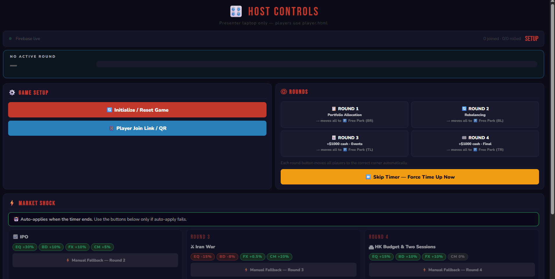
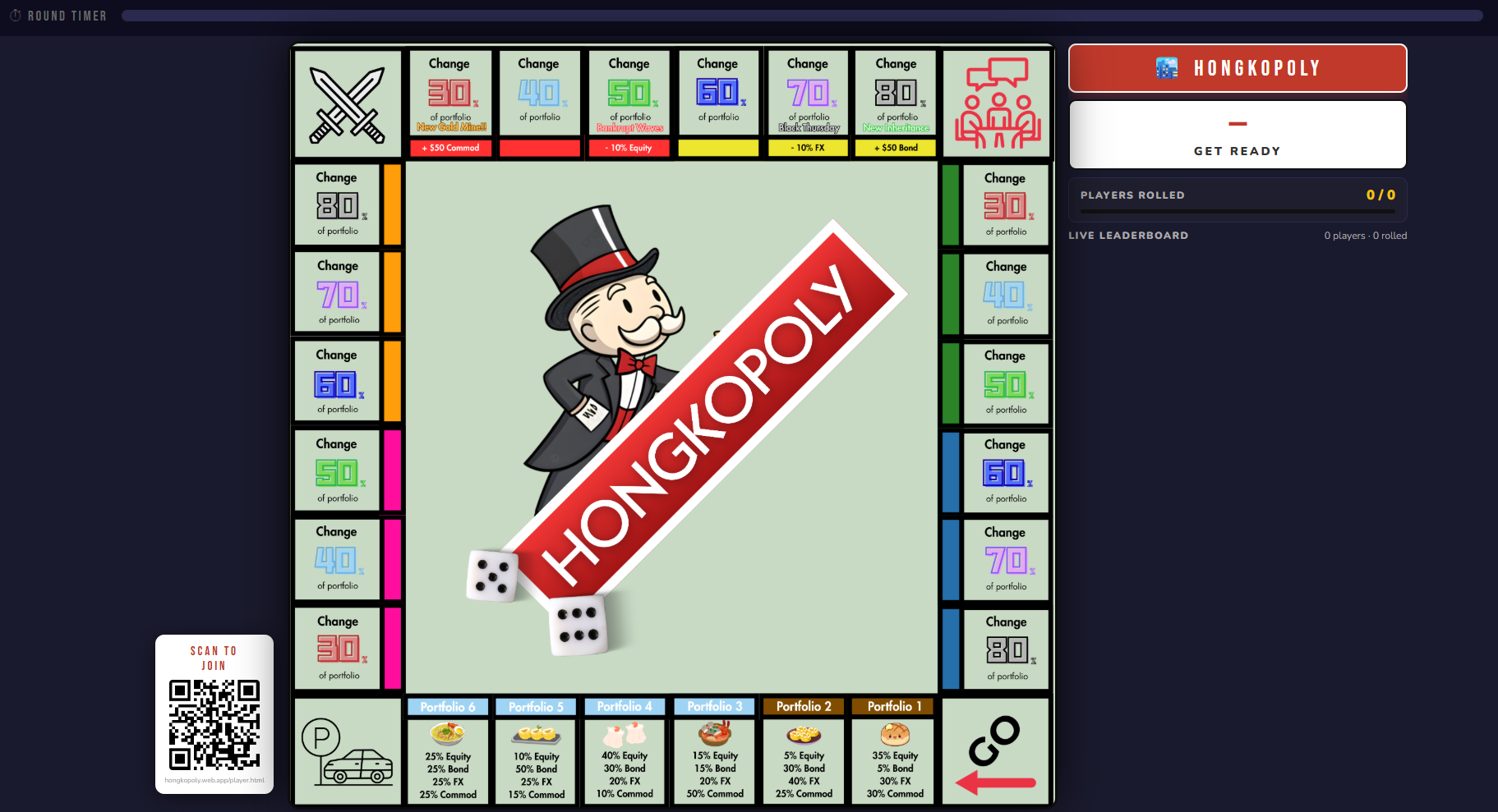

We split the class into 6 teams, and each team will join the game, and as our presentation progress, the results will be revealed. Participants are prompted to invest in the different assets class as a response to current affairs. Feel free to explore how the game work through the links.
That's all! I hope you enjoyed my study guide of the Financial Markets & Investments module. Once again, this is based on my personal experience, and there may be errors that I did not notice. As Heraclitus wisely said, "The only constant in life is change," so the curriculum might have already evolved by the time you read this. Please take this as a guide, not a definitive account!